


Choose your region, country/territory, and preferred language
What is the Polymerase Chain Reaction (PCR)?
Introduction
The polymerase chain reaction (PCR) is arguably the most powerful laboratory technique ever invented. The ease with which it can be done, the relatively low cost, and it’s unique combination of specificity and sensitivity coupled with great flexibility has led to a true revolution in genetics. PCR has opened doors to areas hidden to all but a few for most of the history of genetics. Yet, along with the everyman power of PCR has come a tacit assumption that everyone knows how to do it and understands it. My experience is that this is not the case. There is a great deal about PCR that most practitioners do not know and many other things that they should know better than they do. The advent of kinetic, or Real-Time PCR has served to add yet another dimension to this cognitive dissonance, particularly in the realms of experimental as well as primer and probe design along with optimization of experimental conditions. Moreover, as correctly pointed out by Bustin [1] “The comparative ease and rapidity with which quantitative data can be acquired using real-time RT-PCR assays has generated the impression that those data are reliable and can be subjected to objective analysis.” What has occurred in fact is an even higher level of sophistication that has either been taken for granted or ignored entirely.
In this tutorial the fundamentals of the polymerase chain reaction are discussed.
A Brief (Very) History of PCR
Any attempt to document the development of the polymerase chain reaction will encounter nearly as much myth as science. The strict fact, at least as reiterated in the literature, is that the polymerase chain reaction was conceptualized and operationalized by Kary Mullis and colleagues at Cetus Corporation in the early 1980’s [2]. The method was first formally presented at the American Society of Human Genetics Conference in
October of 1985 and the first clinical application for PCR, an analysis of sickle cell anemia, was published the same year [3]. In its initial form, PCR was tedious and labor intensive. However, the advent of a method by which a specific DNA sequence could be isolated from its genomic context and amplified virtually without limit would not long remain a tool of graduate student and post-doc abuse. The breakthrough came with the isolation and purification of thermostable DNA polymerases [4]. This allowed for PCR to be automated and soon the first programmable PCR thermal cyclers appeared on the market. Since that time, PCR has spread to literally every corner of the world and to every conceivable aspect of biology and chemistry. So profound was the impact of PCR that Kary Mullis was awarded the 1993 Nobel Prize in Chemistry, not even ten years after its introduction.
The PCR Reaction Components
Despite the numerous variations on the basic theme of PCR, the reaction itself is composed of only a few components. These are as follows:
- Water
- PCR Buffer
- MgCl2
- dNTPs
- Forward Primer
- Reverse Primer
- Target DNA
- Polymerase
Considering each of these components, we can begin with Water. While it may seem trivial, water can be a source of concern and frustration. Water is present to provide the liquid environment for the reaction to take place. It is the matrix in which the other components interact. For most people and in most labs sterile, deionized water is the choice. However, water purification systems can fail, the cartridges might not get changed often enough, or contaminants may still get through. In order to eliminate this as a potential problem, we have switched to HPLC-grade bottled water for every application in the lab. This includes reagents. Thus, even our gel buffers are made with HPLC-grade bottled water (see www.idtdna.com on-line catalog for purchasing water).
The next component is the PCR Reaction Buffer. This reagent is supplied with commercial polymerase and most often as a 10x concentrate. The primary purpose of this component is to provide an optimal pH and monovalent salt environment for the final reaction volume. Many commercially supplied PCR buffers already contain magnesium chloride (MgCl2). MgCl2 supplies the Mg++ divalent cations required as a cofactor for Type II enzymes, which include restriction endonucleases and the polymerases used in PCR. The standard final concentration of this reagent for polymerases used in PCR is 1.5mM. Sometimes it is necessary to change this
concentration in order to optimize the PCR reaction. For this reason we choose to obtain PCR buffer without MgCl2 and to add it ourselves. 3.0ul of the standard 25mM MgCl2 provided commercially will yield a 1.5mM final concentration in a 50ul reaction volume.
The purpose of the deoxynucleotide triphosphates (dNTPs) is to supply the “bricks.” Since the idea behind PCR is to synthesize a virtually unlimited amount of a specific stretch of double-stranded DNA, the individual DNA bases must be supplied to the polymerase enzyme. This much is obvious. What might not be as obvious is the fact that the PCR reaction requires energy. The only source of that energy is the β and γ phosphates of the individual dNTPs. One useful hint here: while the PCR buffer and the MgCl2 will stand up to repeated freezing and thawing, the dNTPs are a different story. It is best to obtain them commercially as a 10 mM dNTP mix and to immediately aliquot them into smaller working volumes such that only a fraction of the original dNTP supply is ever thawed out at any one time. The remainder remains frozen until needed and should not cause any difficulty.
We will not discuss PCR primers at this point but will consider them in detail below. The next component is, of course, the target DNA. The quality and quantity of the target DNA is important. The phrase “garbage in-garbage out” is apt. The DNA used as the PCR target should be as pure as possible but also it should be uncontaminated by any other DNA source. The PCR reaction does not discriminate between targets. That is, DNA is DNA is DNA as far as the reaction is concerned. Thus care must be taken to ensure that the target DNA only contains the target of interest. As far as target concentration goes, it depends upon both the source and the method. Plasmid DNA is small and highly enriched for the specific target sequence while genomic DNA will usually contain only one copy of the target sequence per genome equivalent. Thus it is necessary to use more of the latter than the former to present a sufficient number of targets for efficient amplification. We have settled upon a maximum of 100ng of genomic DNA for PCR amplifications from a genomic background. For mammalian genomes, this represents about 10,000 genome equivalents in the reaction. For many reactions substantially smaller amounts can be used. Here, it is really a function of how much DNA you have, how easy is it to replace, and how good it is.
Finally, before looking at PCR primers, a few issues surrounding DNA polymerases should be presented. In the very earliest days of the polymerase chain reaction amplifications were carried out using water baths and lab timers and the best available DNA polymerases of the time, Klenow or T4 DNA polymerase. During the essential DNA denaturation step, 94oC or 95oC for up to a minute, the DNA target was rendered single stranded. It also destroyed the polymerase each time so that fresh enzyme had to be added just after each denaturation step. Since the average duration of a PCR cycle is about five minutes, this became a very labor-intensive bottleneck. The answer to this problem was, as are all good solutions, blindingly simple. There exists in nature organisms that are perfectly happy at very high temperatures. Such organisms, called thermophiles or “heat loving”, were defined by Brock as organisms that live all or part of their life cycle above the so-called thermophile boundary which is set at 50-60oC [5]. Williams defined several terms that describe the relationship between temperature and growth rate for thermophilic bacteria [6]. Bacteria that have a temperature optimum above the boundary but will grow over a wide range of temperatures are termed Euthermal while those growing only over a narrow range are termed Stenothermal. In addition, Williams made a distinction between organisms that will only tolerate high temperatures, thermotolerant, and those that actually live and grow above the boundary, thermophilic [6]. Within the latter category are two further refinements. Facultative thermophiles will grow at temperatures below the boundary but obligate thermophiles will not. As noted by Brock, “… it is the temperature range over which a bacterium is able to maintain a population that is important.” [5].Since such organisms cannot continuously resupply their own enzymes it stood to reason that those enzymes must be resistant to high temperatures [7]. The first of these thermophilic organisms to be exploited was the bacterium Thermus aquaticus which resides in the outflows of thermal pools in Yellowstone National Park (Figure 1).
{{Figure image here}}
Figure 1. Photograph of a thermal pool in Yellowstone National Park. The temperature of the water in the pool is at the boiling point for that altitude. As the water in the outflow on the right cools, an orange coloration begins to appear in the water (arrow) and continues downstream for several feet. At the mid-point of that coloration, the average temperature is 80oC. The organism responsible for the color is Thermus aquaticus. (Photo by Ric Devor).
The DNA polymerase from Thermus aquaticus is stable at 95oC and allowed for automation of the PCR process. The nomenclature rule for enzymes derived from microorganisms is to use the first letter of the genus and the first two letters of the species. Thus, the DNA polymerase from Thermus aquaticus is called Taq.
Since it was first isolated, Taq DNA polymerase has become the standard reagent for the PCR reaction. The gene has been cloned and used to produce the enzyme in non-thermophilic host bacteria so both native Taq, isolated from Thermus aquaticus, and cloned Taq, isolated from expression systems in other bacteria, are commercially available. In addition, a number of other thermal-stable DNA polymerases, isolated from other thermophilic species, have become available. Among these are enzymes from Pyrococcus furiosus (Pfu polymerase), Thermus thermophilus (Tth polymerase), Thermus flavus (Tfl polymerase), Thermococcus litoralis (Tli polymerase aka Vent polymerase), and Pyrococcus species GB-D (Deep Vent polymerase). Each of these, and other, polymerases has a specific set of attributes that can be selected depending upon the application. In general, there are three aspects of a DNA polymerase that should be considered. These are; 1. processivity, 2. fidelity, and 3. persistence.
Processivity refers to the rate at which that polymerase enzyme makes the complementary copy of the template. The standard here is Taq polymerase, which has a processivity of 50-60 nucleotides (nt) per second at 72 oC. The rule of thumb is to simply assume a low-end default processivity for Taq polymerase of 1000 nt per minute bearing in mind that setting your extension times for this assumed value is more than adequate. Many of the other polymerases listed above are slower than Taq. For example, Tth polymerase processivity is on the order of 25 nt per second and others such as Vent and Deep Vent fall in this range as well. However, these enzymes have advantages over Taq polymerase that derive from and compensate for lower processivity. One of the most important of these other features is fidelity. This refers to the accuracy of the complementary copy being made. Taq DNA polymerase has among the highest error rates of the thermophilic polymerases at 285 x 10-6 errors per template nucleotide. Tli polymerase has a proof reading ability that is five-fold better than Taq at 57 x 10-6 errors per template nucleotide and Pfu polymerase also demonstrates fidelity in this range [8]. Finally, the attribute of persistence, which refers to the stability of the enzyme at high temperature, is intimately linked to the other two polymerase attributes. Stability can be measured in terms of how long the enzyme retains at least one-half of its activity during sustained exposure to high temperature. Taq polymerase has a half-life of about an hour and a half at a sustained 95oC. Other enzymes have much longer half-lives. Tli polymerase has a half-life of over six hours and Deep Vent polymerase has shown a half-life of nearly a full day when exposed to a constant 95oC.
As noted, the choice of a polymerase for PCR is application-dependent. For the vast majority of PCR amplifications, the average size of the PCR product (amplicon) is less than 500 base pairs (bp). For this, the error rate of Taq polymerase is negligible and its processivity is ideal. Thus, it is not just historical accident that makes Taq polymerase the reagent of choice for most PCR amplifications but also the fact that, for conventional PCR, it remains the best choice. Many of the other polymerases noted above become the favored choice, often in a mix with Taq, for applications such as long-PCR in which the amplicon is several kilobases long [9]. There, fidelity becomes more of an issue than processivity. Also, Taq polymerase is not an optimum choice for DNA sequencing. In contrast, applications in which there is a need to incorporate non-standard nucleotides such as inosine, deoxyuridine, or 7-deaza-guanosine fare much better with Taq polymerase than with the others because Taq more easily incorporates non-standard nucleotides [10].
Perhaps saving the best until last, DNA polymerases from various species of the genus Thermus have a very unusual property not shared by other DNA polymerases. These enzymes do not possess 3’→5’ proof reading ability whereas other polymerases do possess this ability. The consequence of the lack of 3’→5’ proof reading ability is that Taq polymerase adds a single 3’ nucleotide (Adenosine) on both strands of every amplicon. This 3’ extension permits direct cloning of a PCR product using one of the various commercially available PCR cloning vectors. The DNA polymerases of other species of the genus Thermus also have this property. This includes both Tli and Tth polymerases.
Designing PCR Primers
If all of the components of a conventional PCR reaction discussed above are attended to and can be assumed to be optimal, the success of a PCR reaction will ultimately depend upon the primers and the reaction conditions. Since the latter is dependent upon the former to a large degree, we will here focus on the design of the primers and later discuss reaction conditions.
The purpose of a PCR primer is to specify a unique address in the background of the target DNA. In order to do this, two aspects must be considered. First is the length of the primer and second is the actual sequence of the primer. Regardless of the actual sequence of a PCR primer, its length must be sufficient to guarantee that it will occur in the background target DNA less than once by chance alone. This, then, raises the question, “How long should a PCR primer be?” The answer to this question for any potential target DNA can be determined by a simple statistical exercise.
Let us assume, for the sake of argument and ease of computation, that each of the four DNA nucleotides will occur in the target DNA in equal proportions. That is, at any position in the target each of the four nucleotides has an equal probability of occurrence. Thus, the probability of an A at a specified position is given as p{A}=0.25 and p{A}=p{T}=p{C}=p{G}. Since we assume that this holds for every subsequent position as well, we are doing what is termed sampling with replacement. We also assume that the nucleotide in each subsequent position is independent of the nucleotides in all previous positions. Therefore, the probabilities are independent over the entire length of the target. In order to calculate the probability of any specific dimer, such as AC, we can write a conditional probability as p{C|A} or, the probability of C given that there is an A in the previous position. Since these are independent events by assumption, their probabilities are independent and, therefore, multiplicative. Thus, p{C|A}=0.25 x 0.25 = 0.0625 or (0.25)2. For the trimer ACG the probability is written p{G|AC) = 0.25 x 0.0625 = 0.0156 or (0.25)3. Taking the human genome as our background target, we can estimate the number of times the dimer AC and the trimer ACG would occur by chance alone. The size of the human genome is 3.3 x 10⁹bp (3.3 billion base pairs). If we multiply 0.0625 by 3.3 x 109, the dimer AC will occur in the human genome 206,250,000 times by chance alone. Similarly, the trimer ACG will occur 51,480,000 times by chance alone. Taking this result it is possible to specify an oligomer of length n that will occur in the human genome less than once by chance alone. The n that satisfies this condition is n = 16; (0.25)16 = 2.33 x 10⁻¹⁰[x 3.3 x 109 = 0.77]. Since this is barely less than once, it is useful to “hedge” by making n larger (Table 1). It is for this reason that PCR primers are usually at least 20-mers.
Table 1 Random PCR Primer Sequence Occurrence
| n | (0.25)n | Random Occurrence* |
|---|---|---|
| 1 | 0.25 | |
| 2 | 0.0625 | 206,250,000 |
| 3 | 0.0156 | 51,480,000 |
| 4 | 0.0039 | 12,870,000 |
| 5 | 0.0010 | 3,300,000 |
| 6 | 0.0002 | 660,000 |
| 7 | 0.00006 | 198,000 |
| 8 | 0.000015 | 49,500 |
| 9 | 0.0000038 | 12,540 |
| 10 | 0.00000095 | 3,135 |
| 11 | 0.00000024 | 792 |
| 12 | 0.00000006 | 198 |
| 13 | 0.00000001 | 33 |
| 14 | 3.73 x 10⁻⁹ | 12 |
| 15 | 9.31 x 10⁻¹⁰ | 3 |
| 16 | 2.33 x 10⁻¹⁰ | 0.77 |
| 17 | 5.82 x 10⁻¹¹ | 0.19 |
| 20 | 9.09 x 10⁻¹³ | 0.003 |
| 25 | 8.88 x 10⁻¹⁶ | 0.000003 |
*assuming a genome size of 3.3 x 10⁹bp
This exercise is applicable to any DNA source and can be modified both for the size of the genome and the actual G/C:A/T content of that genome. However, it is sufficient to note that a specified PCR primer of at least 20nt length will stand a very good chance of being unique. Remember, too, that a PCR amplification requires two such primers that stand a specified distance apart. The chances of writing two 25-mer sequences that lie exactly 476bp apart and having that exact combination occur by chance somewhere other than where you got those sequences is nearly zero! Thus, length and proximity serve to guarantee a unique address in your target DNA.
Knowing that two 25-mers separated by a known, fixed distance will suffice for a unique address, how do you choose the sequences of those 25-mers? Clearly, not just any old pair of 25nt sequences will do for PCR. Here, we must now consider the actual sequence attributes of melting temperature (Tm) and secondary structures. The term melting temperature comes from the term melt that has been used to refer to the thermal denaturation of duplex nucleic acid strands. In the classic usage, a melting curve can be determined for any nucleic acid duplex; i.e., DNA::DNA, RNA::RNA, or DNA::RNA. The amount of dissociation of the strands can be measured by a spectrophotometer over a range of increasing or decreasing temperatures. The mid-point of the melting curve is defined as the Tm (Figure 2). As a first-order approximation, the melting temperature of an oligonucleotide of length n used to be figured by adding 2oC for each A or T and 4oC for each C or G, the Wallace Rule [11]. The difference reflected the extra Watson- Crick bond that a C:G pair would have versus an A:T pair under the assumption that it required more energy to break the former than the latter. This calculation also assumes a salt concentration of 0.9M. Thus, the sequence CATGGTACTTATCGC would be calculated to have a Tm of 44 oC simply based upon the numbers of each base in the sequence.
{{Figure image here}}
Figure 2. Hypothetical nucleic acid duplex melting curve. The inflection point of the curve, as determined by the change in optical density between duplex (0.0) and complete denaturation (1.0), is the Tm.
Beginning with the work of Howley et al. and the work of Breslauer et al. it became clear that Tm was not simply a matter of the different nucleotides and their Watson-Crick bonds [12, 13]. The concentration of monovalent cations and, later, divalent cations as well as the type of nucleotide on either side, the nearest-neighbors, played a substantial role in the actual Tm value of an oligonucleotide [14, 15]. From these, and other, studies a much more sophisticated sequence-specific view of oligonucleotide Tm has emerged along with far more accurate methods of estimation.
Another aspect of sequence-specific thermodynamic effects is the concept of stability. It may sound odd at best to suggest that an oligonucleotide only 24 bases long actually has domains in it but that is precisely the case, if only in a heuristic sense. The first domain is composed of the entire length of the oligonucleotide and its specific base sequence. This can thought of as the address domain. That is, the particular length and order of bases that specify a unique address in the target DNA. Within this particular, presumably unique sequence of bases, however, are two additional critical regions. The first of these is composed of the last six nucleotides, the 3’-end hexamer.
DNA polymerases require only a six base duplex to bind and to begin extending. Rychlik notes that the process of binding and extension happens very quickly once a stable duplex is established [16]. Thus, the more stable a 3’ terminal duplex is, the more frequent the binding and extension events. While this would seem to be a desirable situation that should be useful in PCR primer design, the reality is that very stable 3’ terminal duplexes in primers will actually reduce the efficiency of the amplification reaction as measured by the proportionate yield of the correct amplicon. This relationship is shown in Figure 3. The reason for this counter-intuitive result is that primers form transient duplexes and only some of these are with the target of interest. If transient
{{Figure image here}}
Figure 3. Relationship between the stability of the 3’ hexamer of a PCR primer, as measured by increasing ΔG, and the efficiency of the PCR amplification, as assessed by per cent yield of the desired amplicon.
duplexes are formed by sub-sequences of the primer anywhere but the 3’ end there is no consequence. If the transient duplex is formed by the 3’ terminal hexamer, there is sufficient time for DNA polymerase to bind and begin extension. Since many of these 3’ terminal duplexes are false priming events, reagents are being consumed and the overall efficiency of the amplification is decreased. Following Rychlik, the ideal primer design will shift the “stability burden” more 5’ and seek to lower the relative stability of the 3’ terminal hexamer.
How can one visualize the overall stability pattern of an oligonucleotide? Taking a first-order approximation of nearest-neighbor transition free energy values, a 25 base primer sequence can be assessed by breaking it down into overlapping five nucleotide “words.” For example, the sequence CCGGCGCAGAAGCGGCATCAGCAAA is composed of 21 overlapping 5nt words; e.g., CCGGC, CGGCG, GGCGC, GCGCA, etc. If the transition free energy values provided in Table 2 are used the stability of the first pentamer is ΔG = -3.1 + -3.6 + -3.1 + -3.1 = -12.9. The stability of the pentamer AGAAG is ΔG = -1.6 + -1.6 + -1.9 + -1.6 = -6.7. In thermodynamic terms a ΔG value of –12.9 is much more stable than is a value of –6.7. All other things being equal, thermodynamic stability, as measured in
PCR Yield (%)
100
75
50
25
3’ Terminal Duplex
G
terms of ΔG values, increases as the value becomes more negative. A negative ΔG means that energy must be added in order to disrupt the duplex and, thus, the duplex remains stable at higher temperatures. Therefore, it would be better to have the latter stability at the 3’ end than the former in order to avoid as much interference from transient duplexes as possible. The complete stability profile of the 25-mer is shown in Figure 4. This is a good profile because the stability burden is shifted into the more 5’ parts of the address domain while keeping the 3’ end stability reasonably low.
Table 2
Free-energy values of Nearest Neighbor Transitionsa
Second Nucleotide
First Nucleotide dA dC dG dT
dA -1.9 -1.3 -1.6 -1.5
dC -1.9 -3.1 -3.6 -1.6
dG -1.6 -3.1 -3.1 -1.3
dT -1.0 -1.6 -1.9 -1.9
aat 25oC
{{Figure image here}}
Figure 4. Stability profile of a 25-mer oligonucleotide based upon nearest neighbor free-energy transitions. Here, the stability burden, identified by higher ΔG values, is shifted internally and 5’ while the 3’ end stability is kept relatively lower.
The final domain of the PCR primer is, simply, the 3’-terminal nucleotide. Regardless of how ideal the rest of the primer may be, if there is a mismatch between the primer and its target for the 3’ terminal nucleotide, there will be no extension of the polymerase. Since it is impossible to know where and how many mismatches may exist
CCGGCGCAGAAGCGGCATCAGCAAA
G
-12
-10
-8
-6
between the primer sequence and the actual target DNA sample, it is somewhat comforting to know that overall genomic mutation rates are low for most organisms and that a 3’ terminal nucleotide mismatch should be rare. On the other hand, it is also good to be aware that it can happen.
To this point the discussion of primer design has focused on the interaction of the primer, or primers, with the target DNA. Now, we must consider the interactions that can occur between a primer and itself and between two primers. This is the arena of secondary structures. Secondary structures can come in two forms; hairpins and primer duplexes. The latter is further composed of homo-duplexes and hetero-duplexes. The ideal PCR primer should exist in an unblocked linear state in order for it to efficiently bind to its target (i.e., anneal). Any compromise of that unblocked, linear state will rapidly decrease the ability of the primer to bind. Since DNA has only a four-letter alphabet and since the four letters occur in two complementary pairs, it is nearly impossible to create a DNA sequence on the order of a PCR primer in which there will not be some degree of self-complementarity. It is even less likely that two PCR primers will fail to exhibit some degree of cross-complementarity. The only important question to be answered in this context is, “Will the inevitable secondary structures be stable at the temperature of the desired reaction?” Put another way, will the ΔG value of any of the possible secondary structures be negative or positive at the projected reaction temperature? Again, a negative ΔG means that additional energy in the form of heat is required to destabilize the secondary structure and a positive ΔG means that the secondary structure is not stable at the projected reaction temperature.
Primer Design Software
Assessing secondary structures can be done by hand but it is tedious and can be inaccurate to say the least. Fortunately, there is software available that will assess secondary structures and will do so in the context of the most accurate Tm estimates available. The software is OligoAnalyzer 3.0 and it is accessible on-line as part of IDT’s SciTools software at www.idtdna.com. The OligoAnalyzer tool is one of several tools that includes a PCR primer and probe picker. The primer/probe selection tool will be discussed below as well.
Once a primer sequence is chosen, OligoAnalyzer 3.0 provides the user with virtually all of the information necessary to assess the quality of that choice short of actually using it in an assay. The first screen allows the user to enter the candidate primer sequence. As part of the entry screen the user is able to specify any possible modification. The choices include standard DNA or RNA sequences, mixed bases, and an extensive list of 5’, 3’, and internal modifications (Figure 5A). In addition, the analysis of the proposed sequence can be done in various oligo and salt concentrations. The defaults for those variables are selected to represent a conventional PCR assay. Once the sequence is entered, the first step is “Analyze.” Here, information is returned that includes the length of the input
sequence, the complement of the input sequence, its GC content, its melting temperature, molecular weight, and extinction coefficient (Figure 5B).
Secondary structures in your sequence are then assessed by first selecting “Hairpin.” This loads the primer sequence into the mFold sub-routine. mFold is a nucleic acid folding program written by Dr. Michael Zuker [17]. Here, the interactive display will allow for the user to specify the type of nucleic acid (DNA or RNA) and the type of sequence (linear or circular). In addition, there are several options that can be specified as analysis context. These are the temperature at which the evaluation is done, the monovalent (sodium) and divalent (magnesium) ion concentrations, and the more esoteric option of sub optimality (Figure 5C). In general use for PCR (i.e., every-day pragmatic use), the only variables that should always be specified are the evaluation temperature, which should be set to the expected annealing temperature of the PCR assay, and the Magnesium concentration, usually 1.5mM. Once these are entered the sub-routine will provide hairpin structures along with relevant thermodynamic information (Figure 5D). The most useful piece of information contained in the output is a ΔG value for each hairpin. It is important to remember that that number is the ΔG for that hairpin at the assay temperature! A positive ΔG means that the hairpin will not be stable at the assay temperature even though it may be at lower temperatures. Negative ΔG means that the hairpin will be stable at the assay temperature. However, there is stable and, then, there is stable. A value for stability must be considered in the context of the actual assay. A hairpin in isolation in the computer program provides a useful data point but that hairpin will exist in reality in a PCR assay in which the hairpin is competing with the potential DNA::DNA duplex formed by the primer and its target. As a rule-of –thumb, for values in the range –1.00 < ΔG < 0.00, the bi-molecular reaction will out compete the uni-molecular reaction. For values in the range –2.00 < ΔG < -1.00 it’s a judgment call but values exceeding –2.00 should be a cause for concern.
After the hairpin assessment is made, the sequence can be fed into the “Self-Dimer” sub-routine. Here the evaluation of the output is somewhat less subjective. The self-dimer sub-routine will slide the primer over itself as a pair of linear sequences and calculate the ΔG value of every potential self-dimer. The output is provided with a maximum possible ΔG value (Figure 5E). Here, the user assessment involves comparing the calculated ΔG values to the maximum ΔG. Again, a rule-of-thumb guide is that calculated ΔG’s above 10% of the maximum ΔG will be a potential problem. The user should also be aware of where in the primer sequence the problem is. This will aid in selecting a new sequence, if necessary. If the major problems are on one end or another, especially if it is on the 3’ end, eliminating the potential problem could be as simple as moving the sequence a few bases to the left or right. Of course, when this is done, the entire analysis should be done over starting with “Analyze.”
The final two options in OligoAnalyzer 3.0 are hetero-dimer and BLAST. Heterodimer provides the same type of information as self-dimer except that the user enters both members of a primer pair in order to assess potential dimeric interactions between the two. Heterodimer output looks exactly like the self-dimer output shown in Figure 5E and interpretation of the ΔG data is also the same.
BLAST stands for Basic Local Alignment Search Tool and is supported by the National Center for Biotechnology Information [18]. There are several BLAST options available and these are covered comprehensively in any one of the available Bioinformatics books such as Baxevanis and Ouellette [19], Mount [20], Campbell and Heyer [21], and Krawetz [22] to name a few. The version that OligoAnalyzer links to is called “Short nearly exact match.” The logic of BLAST is to take an input sequence, either nucleic acid or amino acid, break it down into “words” of 11nt or 7aa, and search the entire database for matches. Once a match is found, the program will attempt to extend the match beyond the limits of the word. The more the words can be extended the greater the overall match of the input sequence to the object sequence. BLAST output, then, consists of a listing of all matches found, up to a certain number that can be specified by the user, along with an alignment score and the e value. It is this value that must be attended to along with the source of the object sequence deemed to match the input, or query, sequence. Simply put, the e-value is the likelihood that the match found occurred by chance alone. As the e-value approaches zero, the likelihood of a chance match correspondingly approaches zero. The source of the object sequence of a match is also important. If the target DNA of the PCR assay is the mouse genome and some of the matches are from E. coli or Arabidopsis- who cares! This is most likely to happen in the short nearly exact match option used for primers and in the standard nucleotide-nucleotide BLAST option if the input sequence is short, say, less than 50nt. As long as the primer sequence gives a good match for mouse the rest is irrelevant since there shouldn’t be any Arabidopsis DNA in your mouse samples anyway. On the other hand, if the primer sequence pulls up seventy-five matches from all over the mouse genome, that is a problem and the primer sequence should be re-thought.
Clearly, the on-going discussion of primer design indicates that there is a lot to think about when choosing a PCR primer pair. Fortunately, there is a software option in ITD’s BioTools that does a great deal of the thinking for you. This option is PrimerQuest.
Primer Quest is designed to take an input sequence (cut and paste) in FASTA format and search that sequence for optimal primer sets using a set of optimizing parameters. The cardinal parameters are primer length, GC content (%), and Tm. Defaults are 24nt, 50% GC, and a Tm of 60.0oC. Amplicon size will vary according to the primer pairs selected. The logic of Primer Quest involves selecting all possible forward and reverse primers within the input sequence and, then, prioritizing based upon all of the design considerations discussed above. Suboptimality is assessed on the basis of deviations from optimal parameters. Deviations are assigned penalty weights that reflect the degree of deviation from optimal. For example, a candidate primer sequence that is 24nt long with a Tm of 59.6 oC and 45.8% GC content will be assigned a higher penalty than a 24-mer whose Tm is 59.9 oC with a 50.0% GC content. In such a case the latter primer will be regarded as a better candidate than the former. In addition, however, 3’
{{Figure image here}}
Figure 5. Screen sequence from IDT OligoAnalyzer 3.0. See text for discussion.
end stability is assessed as well such that the former primer, while not as optimal as the latter on the three cardinal parameters, may have a better stability profile than the latter and would be given a higher priority. The final phase of selection is then to pair all possible forward sequences with all possible reverse sequences and to prioritize the pairs with respect to joint optimality that includes the cardinal parameters and primer dimer assessment. Of course, this is all done in a matter of seconds and up to 50 primer pairs may be reported (default is five pairs).
Primer Quest can be instructed to select PCR primer pairs, PCR primer pairs with an internal probe sequence, either Forward or Reverse sequencing primers, or probe sequences only. There are set up options in which the user can alter default selection parameters. These are found under the Standard and Advanced set up screens. In practice, only the three cardinal selection parameters (primer length, GC content (%), and Tm) are usually altered. There are other user-specified options in the Advanced Screen that are very useful though. The user can paste in a sequence and then choose only certain regions within that sequence for the primer search. This can be done either by excluding part of the sequence or including part of the sequence. For example, consider an input sequence that is 4500bp in length. Under Basic and Standard the entire sequence is searched. Under Advanced the user may select only part of the sequence, say, a 400bp segment beginning at nucleotide 253, for the search. This is specified by the user as 253,400 which means search only the 400 bases upstream from position 253 inclusive. Similarly, the same region can be excluded using the same specification, 253,400. Another important user-specified option is to force a primer pick. This is used when one of the primers must be a certain sequence in a specific location. It can also be used to pick a probe with both PCR primers fixed.
Finally, when primers are chosen, whether under default or user-specified conditions, the primers sequences can be analyzed for secondary structures as in OligoAnalyzer and can be input to BLAST. There is much more to PrimerQuest than has been discussed here. The best advice for learning and becoming comfortable with any of the BioTools software is to simply log on and explore them. There is no penalty for asking the most useful question, “What happens if…?”
The PCR Reaction Itself
Assume the perfect PCR reaction. The water is HPLC-grade, the buffer, MgCl2, dNTPs, and polymerase are brand new, the target DNA is as clean as it can get, and you have designed an optimal primer pair. What’s next? The first thing is to specify the reaction conditions. PCR is a three step cycling process. The first step is to denature the target DNA so as to make it single-stranded and open up the complementary sequences of the primers. This is routinely done at 94oC or 95oC for up to one minute with 30 seconds being the norm. The second step is to choose a primer annealing temperature, Ta. The melting temperature of the primers determines this temperature. The usual place to set the Ta is about 2 oC lower than the lowest Tm of the primers. Thus, if the primer melting
temperatures are 58.5 oC and 59.2 oC, the Ta should be set at 56.5 oC as a starting point. This temperature can, and should, be changed up or down depending upon the results. With regard to duration, the norm is around 30 seconds. This leaves the final step in the cycle, the polymerase extension step. The convention here is to set this temperature to 72 oC, the optimal temperature for Taq polymerase. However, some protocols, especially those for long PCR, lower this to 68 oC to reduce depurination of longer amplicons. The duration of this final step is determined by the length of the amplicon. The rule of thumb is 30 seconds for every 500bp of product. Since most PCR products are less than 500bp, setting the polymerase extension step to 30 seconds works well. For a product of, say, 2,300bp, the duration should be increased to two and one-half minutes to give the polymerase ample time to make the desired product. A generic PCR cycling profile is presented in Figure 6.
Now, the perfect PCR reaction has been assembled, the cycling parameters have been chosen, entered into the thermal cycler, and you have pushed “RUN.” What is actually happening in that tube? A detailed cartoon of the first four cycles of a PCR reaction is presented in Figure 7. During the initial denaturation step there are actually two things happening. First, all of the target DNAs in the reaction are becoming single-stranded. Second, the heat is setting up convection currents in the reaction mix that will start all of the molecules in motion; i.e., Brownian Motion. This motion will ebb and flow during all of the subsequent temperature changes but the motion will never cease. The reaction components will exist in a constant state of mixing. When the denaturation step terminates, the temperature in the tube will be lowered toward the annealing temperature. During this period the primers will be passing through temperature zones in which random transient duplexes will be tried and discarded until, nearing the Tm of the primers, more and more of the primer molecules will find their perfect complement and
{{Figure image here}}
Figure 6. A generic three-step PCR cycle profile.
94oC
72oC
TAoC
Denature
Primer Anneal
Polymerase Extension
will begin to anneal. As the temperature in the tube passes through the Tm range and settles at the Ta temperature, the maximum possible number of primer molecules relative to the number of available targets will have found those targets and will lay down in stable duplexes. At the same time, the DNA polymerase will have been activated by the requisite Mg++ ions and will zero in their preferred substrates, the primer/target duplexes. As these substrates are acquired the polymerase will bind and immediately begin to extend in the 5’→3’ direction from the primer. As the complementary dNTPs are captured and set in place the β and γ phosphates will be released as a pyrophosphate, PPi. This reaction provides the energy needed for the polymerase to move and begin to capture and set the next complementary dNTP. This process will continue up to and through the polymerase extension step albeit at a slower pace and will only cease when the temperature in the tube reaches the level needed for denaturation.
During the very first PCR cycle the only templates available for primer annealing are the target DNAs. As each primer finds its complement on these target DNAs the polymerase will bind and begin to extend. However, on these templates there is no extension stopping point! The polymerase will continue to extend until the denaturation temperature is reached to begin the next cycle. These PCR products form a population of template molecules that are bounded on only one end. There are various terms that can be used to describe these molecules; anchored and semi-bounded are two that we have used. In the second cycle, both the original target DNAs and the anchored DNAs will serve as templates. The former will continue to make anchored products in every cycle of the reaction while the latter will bind the complementary primer and form the first defined PCR amplicon. In every subsequent cycle, the template DNAs, the anchored DNAs, and the amplicons will serve as targets for the PCR primers. The upshot of this is that it is not the actual target DNAs that produce PCR amplicons but, rather, the anchored
DNAs and other amplicons! The implications of this are that the relative mix of forward and reverse anchored DNA molecules is actually a variable that can be manipulated by the relative amounts of forward and reverse primers in the reaction. In the vast majority of PCR reactions the forward and reverse primer concentrations are equal but there are circumstances when it is advantageous to alter the ratios.
In a PCR reaction the amount of template DNA does not change while the number of anchored products increases arithmetically each cycle beginning with cycle 1. Beginning with cycle 2, when the first defined amplicons are formed, the number of defined amplicons increases at a geometric rate. This, then, is the explosive chain reaction from which PCR derives its name (Figure 8). At the end of 35 cycles there are more than 34 billion copies of the amplicon for every copy of the original template sequence in the reaction! Thus, if there are 10,000 copies of the target sequence, there are more than 340 trillion copies of the amplicon.
{{Figure image here}}
Figure 7. The first four cycles of a PCR reaction. On the far left is the reaction mixture of template DNA (one copy) and the mass excess of forward and reverse primers. In Cycle 1 the first of the anchored PCR products (red arrows) are made. In Cycle 2 the first of the primer-defined amplicons (green lines) is made. Note that it is not the DNA template from which the amplicons come but, rather, the anchored PCR products.
{{Figure image here}}
Figure 8. Relative rates of production of anchored products and primer-defined amplicons during a PCR reaction. The rise of anchored products is arithmetic while the rise of primer-defined amplicons is geometric. At the end of a conventional PCR amplification the relative mass ratio of anchored products to amplicons approaches zero.
COPY #
CYCLE #
Template
AnchoredProducts
Amplicons
Cycle Number
1
2
3
4
The picture of PCR amplification shown in Figure 8 is the conventional view and it has been presented in similar form hundreds of times in textbooks and papers. It is important to note that this picture is, in fact, an over-simplification of the actual course of amplicon production in PCR. While the conservation of template molecules and the relatively plodding arithmetic production of anchored PCR products is accurately portrayed, the true shape of the amplicon curve is more complex than meets the eye. The true amplicon production curve is composed of three separate, sequential phases. The first phase is the exponential phase in which the DNA polymerase is madly churning out short, double-stranded amplicons at near-optimum capacity. However, after a time, amplification rate begins to slow and amplicon production enters a log-linear phase sometimes called a quasi-linear phase. Finally, the reaction changes amplification rate again and enters the final, plateau phase. The trajectory of amplicon production is shown in Figure 9 below.
{{Figure image here}}
Figure 9. A typical amplicon production trajectory composed of, 1. an exponential phase, 2. a log-linear phase, and 3. a plateau phase. The red line indicates the curve of a true exponential reaction trajectory.
A number of plausible explanations have been offered to explain the phenomenon of trajectory change in PCR that, theoretically, should not occur under ideal conditions. Among these are; 1. utilization of reagents, 2. thermal inactivation of the polymerase enzyme, 3. polymerase enzyme inhibition via increasing pyrophosphate concentration, 4. reductions in denaturation efficiency, and 5. exonuclease activity. None of these explanations has proved true. Reagent utilization has been eliminated by experiments in which each component was titrated without any apparent effect on trajectory changes. Thermal inactivation has also been eliminated by the observation of trajectory change in the presence of extremely thermal stable polymerases. Pyrophosphate build-up was an attractive idea because these “waste products” of in vitro nucleotide addition; i.e., the reaction dNTP + (dNMP)n → (dNMP)n+1 + ppi wherein each polymerase-catalyzed nucleotide addition results in the irreversible addition of a pyrophosphate, ppi, to the reaction environment, could potentially be inhibiting at late cycle number
Number of Amplicons
Cycle Number
Phase 1
Phase 2
Phase 3
concentrations. However, this idea, too, failed under direct experimental scrutiny. Nor were reductions in denaturation efficiency or exonuclease activities able to pass muster in late cycle conditions. In the end, the answer came from a not-so-simple (except in hindsight) thermodynamic phenomenon.
Kainz [23], who beautifully defined the plateau phase as “attenuation in the rate of exponential product accumulation.”, showed that it is accumulation of the amplicons themselves that induces trajectory change. Once amplicons begin to be produced they exist as double-stranded species that are melted along with the target DNA and the anchored products during the denaturation step. At the end of the denaturation step the reaction is cooled down to the primer annealing temperature. Target DNA begins to re-anneal and, if it is genomic DNA, renaturation follows the familiar Cot curve trajectory with single copy sequences renaturing last. So, too, will the anchored products begin to renature. However, it is the short, renaturing amplicons that begin to cause havoc because they present inviting targets for polymerases. Polymerase molecules will not be affected to any great degree by the relatively small numbers of double-stranded species presented by the renaturaing target DNAs and anchored products. On the other hand the mass increase of double-stranded species represented by the amplicons that have average melting temperatures in the middle to high 80oC ranges will begin to exert an effect on the polymerase population over time. Thus, showed Kainz, the production of amplicons is a self-limiting process.
Related links
Community blog posts
- Infectious disease in 2025: Top threats and alarming trends
- Expression vectors: The what, why, and how
- New bird flu variant has public health officials on edge
- Transcription and translation: 5 differences to know about
- Latest PCR, qPCR, and genomics news headlines
- 5 advantages of Using IDT’s new qPCR master mix
- COVID-19 vs. monkeypox
- 2022 Monkeypox Outbreak
References
- Bustin SA. (2002) Quantification of mRNA using real-time reverse transcription PCR (RT-PCR): trends and problems. J Mol Endocrinol, 29: 23−39.
- Saiki RK, Scharf S, et al. (1985) Enzymatic amplification of β-globin genomic sequences and restriction site analysis for diagnosis of sickle cell anemia. Science, 230: 1350−1354.
- Saiki R, Scharf S, et al. (1985) A novel method for the parental diagnosis of sickle cell anemia. Am J Hum Genet, 37: A172.
- Lawyer FC, Stoffel S, RK, et al. (1989) Isolation, characterization, and expression in Escherichia coli of the DNA polymerase from Thermus aquaticus. J Biol Chem, 264: 6427−6437.
- Brock TD. (1986) Introduction: An overview of the thermophiles. In: Brock TD (ed.) Thermophiles: General, Molecular, and Applied Microbiology. New York: Wiley. 1−16.
- Williams RAD. (1975) Science Progress, 62: 373−393.
- Brock TD. (1997) The value of basic research: Discovery of Thermus aquaticus and other extreme thermophiles. Genetics, 146: 1207−1210.
- Cline J, Braman JC, and Hogrefe HH. (1996) PCR fidelity of Pfu polymerase and other thermostable DNA polymerases. Nucleic Acids Res, 24: 3546−3551.
- Barnes WM. (1994) PCR amplification of up to 35-kb DNA with high fidelity and high yield from λ bacteriophage templates. Proc Natl Acad Sci USA, 91: 2216−2220.
- Seela F, and Roling A. (1992) 7-Deazapurine containing DNA: efficiency of c7GdTP, c7AdTP and c7IdTP incorporation during PCR-amplification and protection from endodeoxyribonuclease hydrolysis. Nucleic Acids Res, 20: 55−61.
- Wallace RB, Shaffer J, et al. (1979) Hybridization of synthetic oligodeoxyribonucleotides to ΦΧ-174 DNA: the effect of single base pair mismatch. Nucleic Acids Res, 6: 3543−3547.
- Howley PM, Israel MF, et al. (1979) A rapid method for detecting and mapping homology between heterologous DNAs. Evaluation of polyomavirus genomes. J Biol Chem, 254: 4876−4883.
- Breslauer KJ, Frank R, et al. (1986) Predicting DNA duplex stability from the base sequence. Proc Natl Acad Sci USA, 83: 3746−3750.
- Owczarzy R, Vallone PM, et al. (1997) Predicting sequence-dependent melting stability of short duplex DNA oligomers. Biopolymers, 44: 217−239.
- SantaLucia JS, Allawi HT, and Seneviratne PA. (1996) Improved nearest-neighbor parameters for predicting DNA duplex stability. Biochemistry, 35: 3555−3562.
- Rychlik W. (1995) Selection of primers for polymerase chain reaction. Mol Biotechnol, 3: 129−134.
- Zuker M. (2003) Mfold web server for nucleic acid folding and hybridization prediction. Nucleic Acids Res, 31: 3406−3415.
- Altschul SF, Gish W, et al. (1990) Basic local alignment search tool. J Mol Biol, 215: 403−410.
- Baxevanis AD and Ouellette FF (Eds.). (2001) Bioinformatics. A Practical Guide to the Analysis of Genes and Proteins. New York: Wiley Interscience.
- Mount DW. (2001) Bioinformatics: Sequence and Genome Analysis. Cold Spring Harbor, New York: Cold Spring harbor Laboratory Press.
- Campbell AM and Heyer LJ. (2002) Discovering Genomics, Proteomics, and Bioinformatics. Redwood City, CA: Benjamin/Cummings.
- Karwetz SA and Womble DD (Eds.). (2003) Introduction to Bioinformatics: A Theoretical and Practical Approach. Totowa, NJ: Humana Press.
- Kainz P. (2000) The PCR plateau phase- towards an understanding of its limitations. Biochem Biophys Acta, 1494: 23−27.